SPAM Twirling

Note

This feature is present only in openqaoa 0.1.4 and above!

State Preparation and Measurement (SPAM) Twirling is a simple error mitigation technique used to remove any preferred direction due to readout noise. It works by diagonalizing the noise associated with measurements by randomly flipping qubits via X gates right before the measurement and flipping the corresponding measured bit classically. A calibration factor from the diagonal noise channel is obtained by measuring quantum circuits initialized in the zero states. As a result, the expectation values of the circuit in the presence of readout noise is much closer to the noise-free one.

For the curious

The technique has been developed theoretically by E. v. d. Berg et al. [1] and by A. W. R. Smith, et al. [2] and implemented within Qiskit as one of their “resilience levels” under the name “Twirled Readout Error eXtinction (TREX)”. Experimentally has been applied by Layden et al. [3] to ensure that the symmetry requirement \(Q(s'| s) = Q(s |s')\) is met. Note that this requirement is specific to the Monte Carlo algorithm and therefore irrelevant to QAOA.

The algorithm

I. Obtain calibration data (ideally for the whole device) under the Bit Flipping Averaging (BFA) subroutine

1. Initialize the circuit in the |000…0> state.
2. Measure under BFA (subroutine)
3. Save the counts and the registers (this is how the measurement string outcomes map to the physical qubits on the device) and all other relevant information to a json (see the code for the exact format).

II. Run the quantum experiment under BFA

1. Calculate calibration factors
2. Prepare the desired quantum circuit
3. Measure under BFA (subroutine)
4. Correct the expectation values by term
5. Combine all corrected terms into the final expectation value

Subroutine: Bit Flip Averaging (BFA) technique

1. Divide the total number of shots into \(n\) batches and for each batch choose a set of qubits to be flipped. Note that since we usually don’t have a very accurate model of the noise and to keep it general, we choose the qubits within each batch uniformly at random.
2. The bit flip before the measurement can be done by applying an X gate, absorbing the X gate into the last layer of RX rotations or propagating it to the front (and then absorbing it into the initial |+> state).
3. The bit flip after the measurement is performed by applying a classical not to the outcome bitstring, which is implemented as changing the keys in the count dictionary.
4. Combine the negated counts from all batches into a single count dictionary which is then used for calculating the calibration factors or estimating the expectation values.

Let's look at a simple example of a 2-qubit system for which the QAOA circuit is:

Under BFA, every batch implements the desired QAOA circuit with single X gates prepended/appended randomly on a subset of the qubits. Considering,as an example, a simple two qubit circuit, there are 3 posibilities for the X gates. They can be applied to the first qubit to the second one or to both:

How to do this within OpenQAOA?

In the workflows, this can be implemented by simply doing:

q = QAOA()
q.set_error_mitigation_properties(
    error_mitigation_technique="spam_twirling",
    n_batches=4,
    calibration_data_location="filename",
)

Internally, OpenQAOA modifies the backend object in order to divide the computation in batches and applies the conditional X gate on a set of qubits choosen uniformly at random

if error_mitigation_properties.error_mitigation_technique == 'spam_twirling':
    backend = SPAMTwirlingWrapper(backend=self.backend,
                                  n_batches=self.error_mitigation_properties.n_batches,
                                  calibration_data_location=error_mitigation_properties.calibration_data_location)

What to expect?

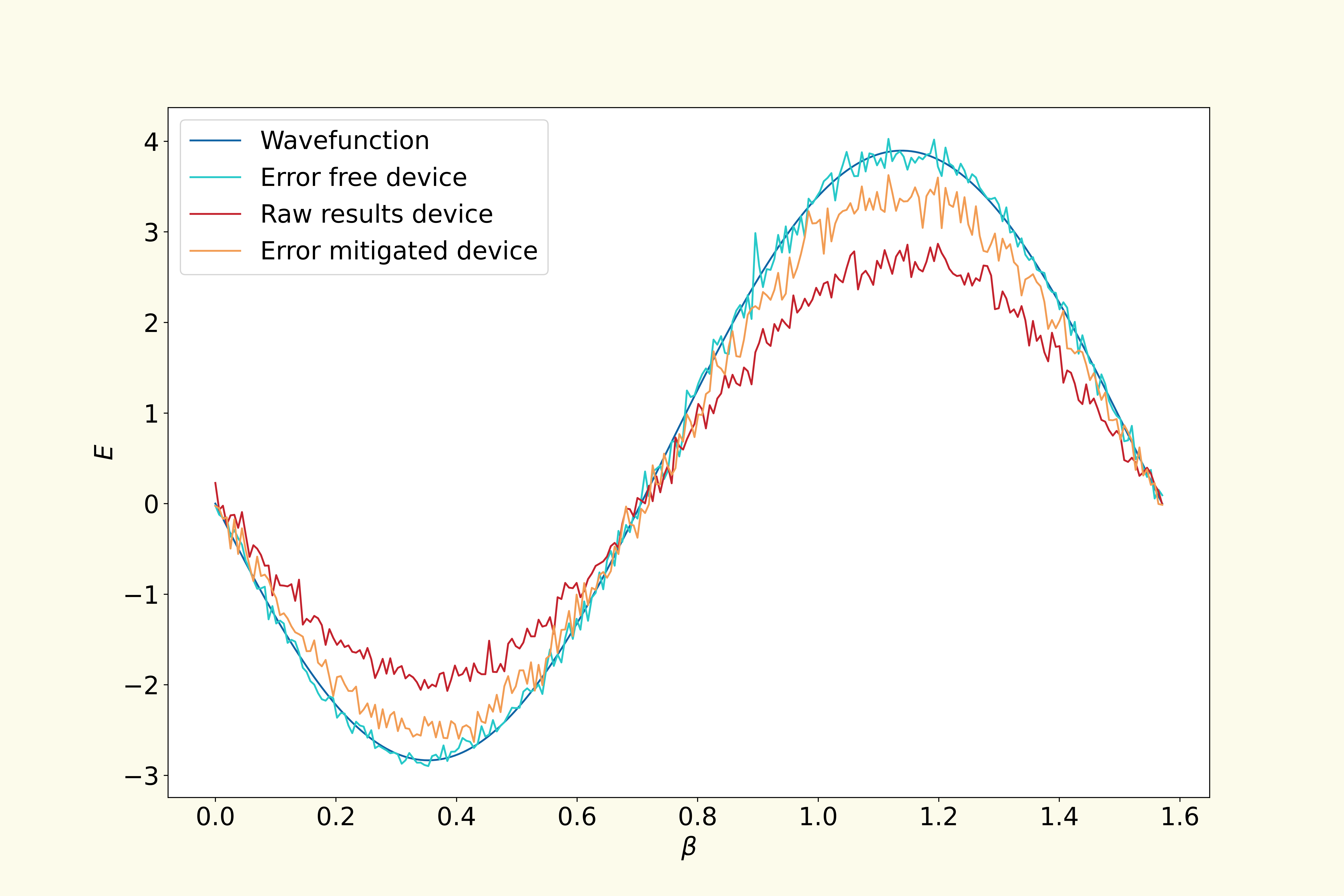
Let's see the technique in practice by solving MaxCut on a u3R graph for n=6 qubits. In this example, we simulate a 7 qubit device using the (noisy) Quantum Virtual MAchine, an emulator developed by Rigetti. We have a total of 1000 shots, we divided them into into 10 batches of equal number of shots (note that the number of batches and shots may be tweaked to improve the result!).

The plot above shows a slice of the landscape at \(\gamma=0.25\) and for various \(\beta\). It is clear that by performing SPAM Twirling we obtain (the orange line) energies much closer to the theoretically simulated ones (dark blue line).

References

---

1. Berg, E., Minev, Z. K., Temme, K., Phys. Rev. A 105, 032620 (2022)
2. Smith, A.W.R., Khosla, K.E., Self, C.N., Kim, M.S., Science Advances, vol. 7, 47 (2021)
3. Layden, D., Mazzola, G., Mishmash, R. V., Motta, M., Wocjan, P., Kim, J.-S., Sheldon, S., arXiv:2203.12497, (see Appendix IV, sec.A2)