Run a QAOA workflow on the cloud - Cloud Simulators

Running a QAOA on a QPU is not an easy task: the QAOA is driven by a classical-quantum loop (see What is the QAOA ) which results in many subsequent executions of quantum circuits on a QPU.

Current hardware is rather noisy, and since customizing QAOAs in general yields more complex circuits let us start east: first, we will submit the QAOA job to a cloud simulator!

Start simple: IBMQ Cloud QASM simulator

The IBMQ QASM simulator is described, on the official IBM docs, as

A general-purpose simulator for simulating quantum circuits both ideally and subject to noise modeling. The simulation method is automatically selected based on the input circuits and parameters.

It will serve us well for this example, since it mimics quite closely they way we interact with any other Quantum Computer: OpenQAOA will generate a sequence of jobs that will be sequentially evaluated by the simulator.

To begin, let's start by creating our usual benchmark problem: an instance of vertex cover:

import networkx
from openqaoa.problems import MinimumVertexCover

g = networkx.circulant_graph(6, [1])
vc = MinimumVertexCover(g, field=1.0, penalty=10)
qubo_problem = vc.qubo

Now that we have the qubo problem, let's focus on the cloud access. To connect to a QPU or to a cloud-based simulator, you will need to authenticate with the desired provider. To check all the available cloud-simulators backends go to the devices page.

First, you will need to have a correctly setup account with IBMQ. Once your account has been created, all you need is your IBMQ token (available with the IBMQ landing page). The recommended way to use your token in OpenQAOA is the following

from qiskit import IBMQ

IBMQ.save_account('MY_API_TOKEN') 

Once we have authenticate we can proceeded with the OpenQAOA workflow

from openqaoa import QAOA, create_device
from qiskit import IBMQ

#Create the QAOA
q = QAOA()

# Load account from disk
IBMQ.load_account() 

# Create a device
ibmq_device = create_device(location='ibmq', name='ibmq_qasm_simulator')
q.set_device(ibmq_device)

q.set_circuit_properties(p=1, param_type='standard', init_type='ramp', mixer_hamiltonian='x')
q.set_backend_properties(init_hadamard=True, n_shots=8000, cvar_alpha=0.85)
q.set_classical_optimizer(method='cobyla', maxiter=50, tol=0.05)

q.compile(qubo_problem)
q.optimize()

Tip

The code above will result in up to 50 optimizer iterations, that is it will submit up to 50 jobs to the ibmq_qasm_simulator device!

Now, let's look into the optimization resuult. First, we can check how many circuits were executed

q.result.evals

yields

{'number_of_evals': 11, 'jac_evals': 0, 'qfim_evals': 0}

This means that we executed 16 circuits within our optimization loop! Indeed, we can retrieve the job ids associated to these execution by tying

q.result.intermediate['job_id']

yields

['6427cf52b072ef0790b5dc25',
 '6427cf56417cad3f6b7f72a0',
 '6427cf5bb072ef0bf8b5dc26',
 '6427cf5f1181d8b3f0a5ad22',
 '6427cf63e6c3c92a8c8cb2e0',
 '6427cf67db7e34d609a98298',
 '6427cf6ce6c3c9dc038cb2e1',
 '6427cf71f2aaddc880a4a9f5',
 '6427cf7522b9b76d3f7845d1',
 '6427cf7a22b9b783547845d2',
 '6427cf7ff2aaddf142a4a9f6']
 ```

These jobs ID are the ones provided by IBM and can be used to retrieve the JSON dump as provided by IBM. We can also easily check the cost value, and confirm that our optimization ended when the tolerance threshold (remember? We set it as `tol=0.05` in the `set_backend_properties()`) was crossed

```Python
q.result.intermediate['cost']

yields

[15.720125,
 20.00975,
 19.1425,
 20.1755,
 19.37075,
 19.310375,
 33.233625,
 19.179,
 14.425375,
 20.4105,
 14.435125]

Finally, what about the optimal state? We can obtain all the pertinent information by executing

q.result.optimized

which yields

{'angles': [-0.372908706525, 0.570235617839],
 'cost': 2.679125,
 'measurement_outcomes': {
  '100000': 2,
  '111010': 203,
  '100110': 24,
  '010110': 24,
  '110110': 242,
  '001110': 11,
  '101110': 195,
  '011110': 81,
  '111110': 587,
  '110101': 221,
  '001101': 24,
  '101101': 246,
  '011101': 204,
  '111101': 612,
  '101011': 212,
  '011011': 228,
  '111011': 612,
  '010111': 176,
  '110111': 603,
  '001111': 78,
  '101111': 554,
  '011111': 553,
  '111111': 1466,
  '111100': 71},
 'job_id': '6427c778b072ef3c75b5dbef',
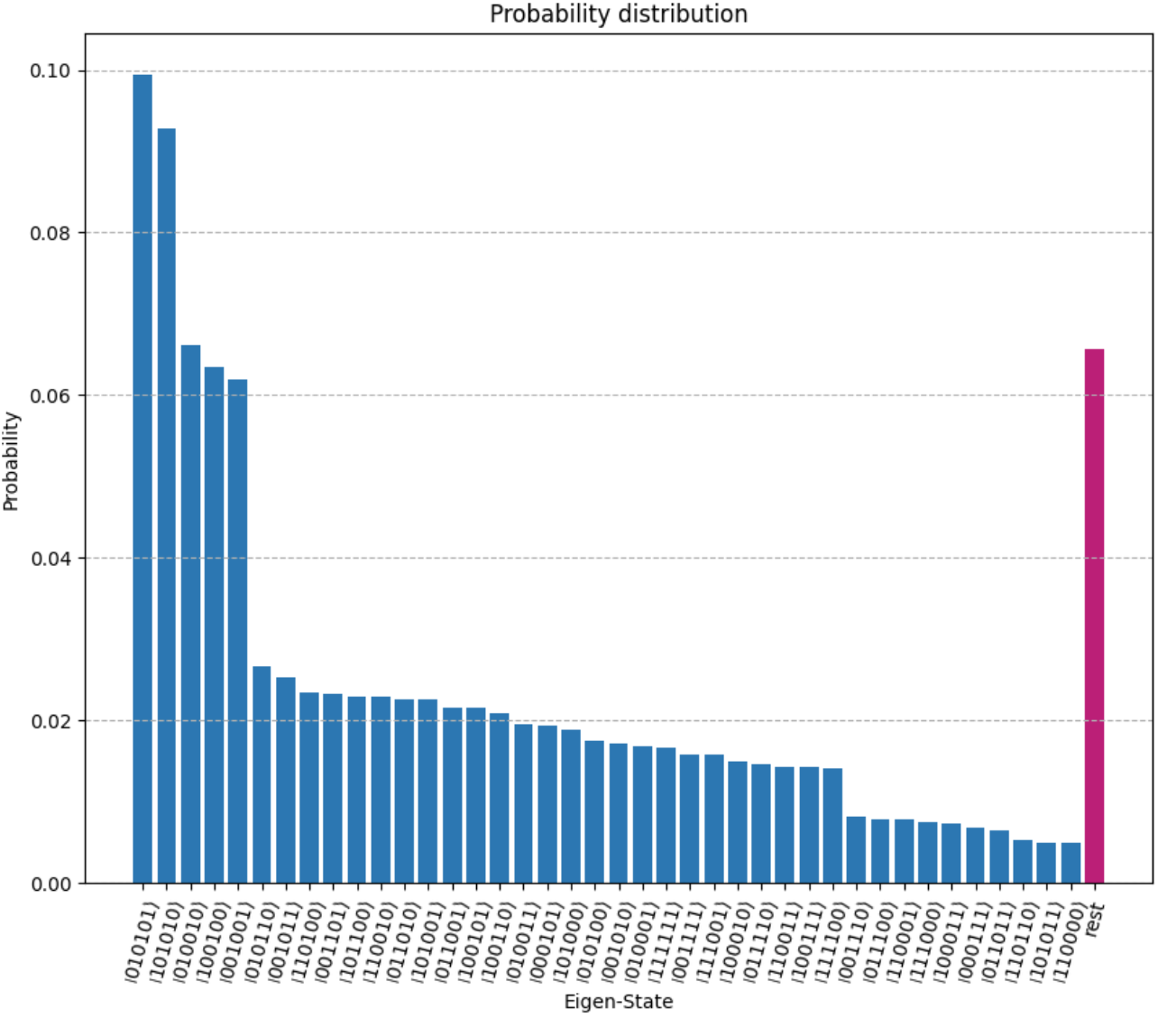
 'eval_number': 14}

For convenience, we can plot the underlying probability distribution

Compare with the exact solution

Now that the jobs have completed and the QAOA is over, let's check the actual result. Within the OpenQAOA utilities there is the convenience function ground_state_hamiltonian(). The function takes as input the cost hamiltonian and, by brute force, finds the optimal solution(s)

from openqaoa.utilities import ground_state_hamiltonian

ground_state_hamiltonian(qubo_problem.hamiltonian)

Which for our benchmark problem gives

{'cost': 3.0,
 'states': ['101010', '010101'])

And we can compare this with the values obtained above:

q.result.most_probable_states

gives

{'solutions_bitstrings': ['010101'], 'bitstring_energy': 3.0}

Which is indeed one of the two minima!