Standard parametrization

The StandardParams class implements the original and conventional form of the QAOA. In every layer of the circuit, the mixer and cost Hamiltonians are applied with coefficients \(\beta(q)\) and \(\gamma(q)\), respectively. That gives a total of 2p parameters for a circuit of p layers to be optimised.

For example, for a depth-2 (p=2) circuit, the unitary operator corresponding to the QAOA circuit would take the form

\[ U(\beta_1,\beta_2,\gamma_1,\gamma_2) = e^{-i\beta^{(2)} H_{M}} e^{-i\gamma^{(2)} H_{C}} e^{-i\beta^{(1)} H_{M}} e^{-i\gamma^{(1)} H_{C}}. \]

Let us take a very simple example where the cost hamiltonian has quadratic terms of the same weight, \(w=2.5\), and biases of \(b=3.5\), namely:

\[ H_C = 2.5 (Z_0Z_1 + Z_1Z_2 + Z_0Z_2) + 3.5 (Z_0 + Z_1 + Z_2). \]

For the curious

This Hamiltonian arises when solving the Minimum Vertex Cover on a 3-nodes ring graph with \(\text{field}=3\) and \(\text{penalty}=10\).

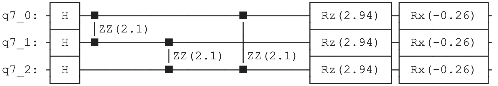
The corresponding \(p=1\) circuit is a layer of Hadamards followed by \(ZZ\) entangling 2-qubit gates, single-qubit rotations around the \(Z\) axis and another layer around the \(X\) axis.

Initialize with standard parameters

Let us initialize the circuit with the custom values of \(\gamma=0.42\) and \(\beta=0.13\).

Then the angles of the \(ZZ\) gate are \(2*\gamma*w = 2*0.42*2.5 = 2.1\), the angles of the RZ gate are \(2*\gamma*b = 2*0.42*3.5 = 2.94\) and the angles of the RX gate are \(-2*\beta = -0.26\) across the whole layer.

We can visualize this using the 'qiskit.statevector_simulator' backend:

Control the bias term

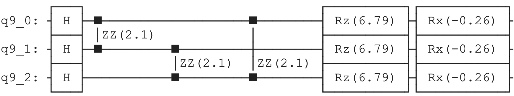
The StandardWithBiasParams class allows for changing the parameter of the RX gate, thus providing a slightly more expressive ansatz for problems with bias terms such as the one of the example above.

Number of parameters

Note that with this parametrization the classical optimizer receives 3 variational parameters. In general, a depth-p circuit will have 3p parameters instead of 2p as in the StandardParams class.

Let us now use this class by setting the circuit properties with

q = QAOA()

q.set_circuit_properties(p=1, 
                        param_type='standard_w_bias',
                        init_type='custom',     
                        variational_params_dict={
                            'gammas_pairs':[0.42], 
                            'gammas_singles':[0.97], 
                            'betas':[0.13]}
                         )

In the circuit model, this looks like:

Hamiltonian without bias terms

If the Cost Hamiltonian does not have a bias term, for example if we are solving MaxCut, using StandardWithBiasParams will result in an error. In those cases simply use the StandardParams class.