Fourier Parametrization
The class QAOAVariationalFourierParams implements a heuristic proposed by Zhou et al. [1] which instead of optimizing for \(\beta\) and \(\gamma\) at each layer aims at finding the amplitudes of their discrete Fourier transforms given by:
where \(i = 0,...,p\).
For the curious
In the paper the series run from 1, while in our notation they run from 0, which changes slightly eq.(1) and eq.(2). Under the hood, we use the Scipy implementation of discrete cosine and sine Fourier transform of type II.
The idea comes from the empirical observation that the optimal parameters are often found to be smoothly varying functions for certain problems (such as the one implemented by the QAOAVariationalAnnealingParams class). Hence, it should be possible to use a reduced parameter set consisting of only the lowest \(q\) frequency components of those functions. Clearly, for \(q\geq p\) we have the full expressivity of the original parameter set (i.e. the \(\beta\) and \(\gamma\)). In this parametrisation, for fixed \(q\), the optimisation problem therefore becomes that of finding the optimal Fourier components \(v_k\) and \(u_k\).
In [1], the authors show that certain variants of this basic Fourier parametrisation can perform significantly better than a randomised brute force search through parameter space, for MaxCut problems on 3-regular and 4-regular graphs.
Number of parameters
The depth of the circuit is still linear in the number of layers, \(p\). The advantage is in the smaller number of variational parameters to be optimized, as long as \(q \leq p\).
Initialize with fourier parameters
Let us once again take the cost Hamiltonian to be \(H_C = 2.5 (Z_0Z_1 + Z_1Z_2 + Z_0Z_2) + 3.5 (Z_0 + Z_1 + Z_2)\) and construct a circuit of 4 layers (p=4). In the standard parametrization this would give \(2*4 = 8\) variational parameters. The fourier parametrization, however, allows to work with less. Let's set \(q=2\), giving only \(4\) parameters to be optimized. We can further specify the initial values of those using the custom initialization, for example with the following:
q.set_circuit_properties(p=4,
                         q=2,
                         param_type='fourier',
                         init_type='custom',
                         variational_params_dict={
                             "u":[0.1, 0.2],
                             "v":[0.9, 0.8]}
                         )
As a circuit, this looks like:
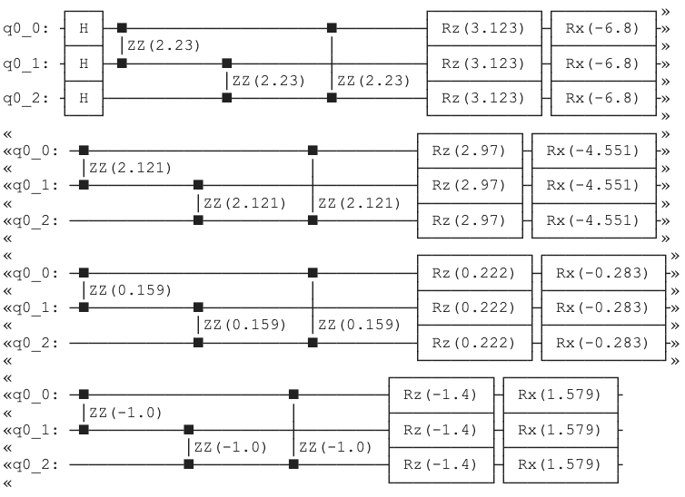
Let us now understand how the custom values we set for u and v translate to the rotational angles we see in the circuit above.
For example, the RX rotation between qubit 1 and 2 in the first layer is obtained by evaluating eq.(2) for i=0, p=4, q=2 and then simply multiplying by 2, as conventional.
This simplifies nicely since \(\cos(0)=1\) and we are left only with a sum over the chosen values of v which gives
For another, a bit more involved, example let us focus on the ZZ rotation between qubits 0 and 1 in the 3rd layer. This comes from evaluating eq.(1) for i=3, p=4, q=2 and then multiplying by the weight of the quadratic term of the cost hamiltonian and by 2, as conventional.
After substituting for the weight and the parameters we chose for u and after expanding the sum, we arrive at
which after simplifying gives
Indeed, this is what we see in the brackets next to this gate.
Fourier with ramp
When the fourier parametrization is initialized with ramp, the optimization starts from \(\vec{v} = \vec{u} = [0.35, 0, 0, ..., 0]\) where the length of the vectors is \(q\). This is because at a single layer, \(p=1\), and no user-specified time, the standard parameters \(\beta\) and \(\gamma\) are 0.35.
Control the bias terms
The class QAOAVariationalFourierWithBiasParams extends upon the above by allowing for an additional parameter controlling the single qubit rotations around the Z axis, analogous to what StandardWithBiasParams implements.
One way to use this class is by setting the circuit properties as:
q.set_circuit_properties(p=4,
                         q=2,
                         param_type='fourier_w_bias',
                         init_type='custom',
                         variational_params_dict={
                             "u_pairs":[0.1, 0.2],
                             "u_singles":[0.5, 0.6],
                             "v":[0.9, 0.8]}
                         )
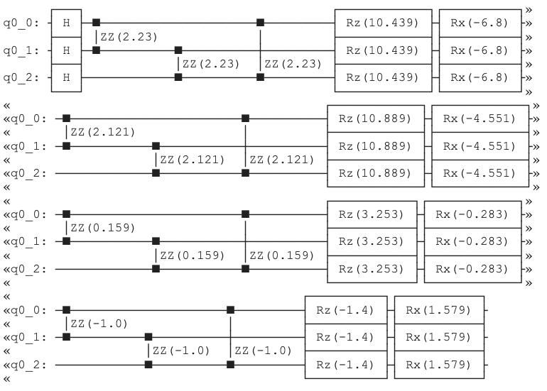
Since we kept the parameters controlling \(\beta\) and \(\gamma\) same as before and only gave new parameters for the single qubit rotations around the Z axis, the circuits look identical apart from the RZ gates.
Number of parameters
When using the QAOAVariationalFourierWithBiasParams class the number of parameters to be optimized is \(3q\).
Control all terms
The class QAOAVariationalFourierExtendedParams, similarly to the ExtendedParams class, unlocks the full flexibility of the ansatz for this particular parametrization.
It can be used with the following piece of code:
q = QAOA()

q.set_circuit_properties(p=4,
                         q=2,
                         param_type='fourier_extended',
                         init_type='custom',
                         variational_params_dict={
                             "u_pairs":[[0.11, 0.12, 0.13], [0.21, 0.22, 0.23]],
                             "u_singles":[[0.51, 0.52, 0.53],[0.61, 0.62, 0.63]],
                             "v_pairs":[],
                             "v_singles":[[0.91, 0.92, 0.93], [0.81, 0.82, 0.83]]}
                         )
Number of parameters
Care must be taken when using the QAOAVariationalFourierExtendedParams as the number of variational parameters scales linearly with n. As shown above, for 3 qubits circuit, \(n=3\) with \(q=2\) and the standard X mixer, the number of parameters is \(n*q*3=18\). Although this is still less than for the ExtendedParams class, as long as \(q<p\), it can result in long optimization times.
References
- L. Zhou, S. Wang, S. Choi, H. Pichler, M. D. Lukin, Phys.Rev.X 10, 021067 (2020) Quantum Approximate Optimization Algorithm: Performance, Mechanism, and Implementation on Near-Term Devices, https://arxiv.org/abs/1812.01041.