Traveling Sales Person Problem

The Traveling Sales Person Problem requires to find, given a list of cities and the distances between each pair of cities (or the cities coordinates), the shortest possible path that visits each city exactly once and returns to the origin city. Additionally, one can also specify how cities are connected together, this can be represented as a graph (directed or not).

The Cost Function

Given a graph \(G=(V, E)\), with \(N=|V|\) vertices, the cost function to minimize for the Traveling Sales Person Problem is given by

\[ C(\textbf{x}) = C_A(\textbf{x}) + C_B(\textbf{x}) . \]

• \(C_A\) is the loss function associated to the Hamiltonian path problem. The problem is as follows, starting at some node and traveling only from existing edges on the graph, can we visit all nodes in the graph without ever returning to a visited node. The variables \(x_{v,i}\) represent the node \(v\) selected at the \(i^{th}\) position. The cost function has three components, each node must be selected once, each position must have one associated node, two consectuive nodes in the selection \(x_{u,i}\) and \(x_{v,i+1}\) should have an associated edge in the given graph (a penalty is applied if \((u,v) \notin E\)). The Hamiltonian path cost function is given by

\[ C_A(\textbf{x}) = A\sum_{v=1}^{n}\left(1-\sum_{j=1}^{N}x_{v,j}\right)^2 + A\sum_{j=1}^{n}\left(1-\sum_{v=1}^{N}x_{v,j}\right)^2 + A\sum(u,v)\notin E \sum_{j=1}^{N}x_{u,j}x_{v,j+1}, \]

where \(A>0\) is a constant, \(N+1\) is interpreted as \(1\). It is easy to see that \(C_A\) is zero if and only if each vertex is included exactly once and adjacent vertices are associated to an edge on the initial graph.

• \(C_B\) is the loss function associated with the distance between cities, penalizing a Hamiltonian cycle that would be longer than another. The cost function is given by

\[ C_B(\textbf{x}) = B \sum(u,v)\in E W_{uv} \sum_{j=1}^{N}x_{u,j}x_{v,j+1}, \]

where \(B>0\) is a constant and \(W_{uv}\) is the weight of each edge. \(B\) should be small enough so it's never favorable to violate the first constraint \(C_A\).

Traveling Sales Person Problem in OpenQAOA

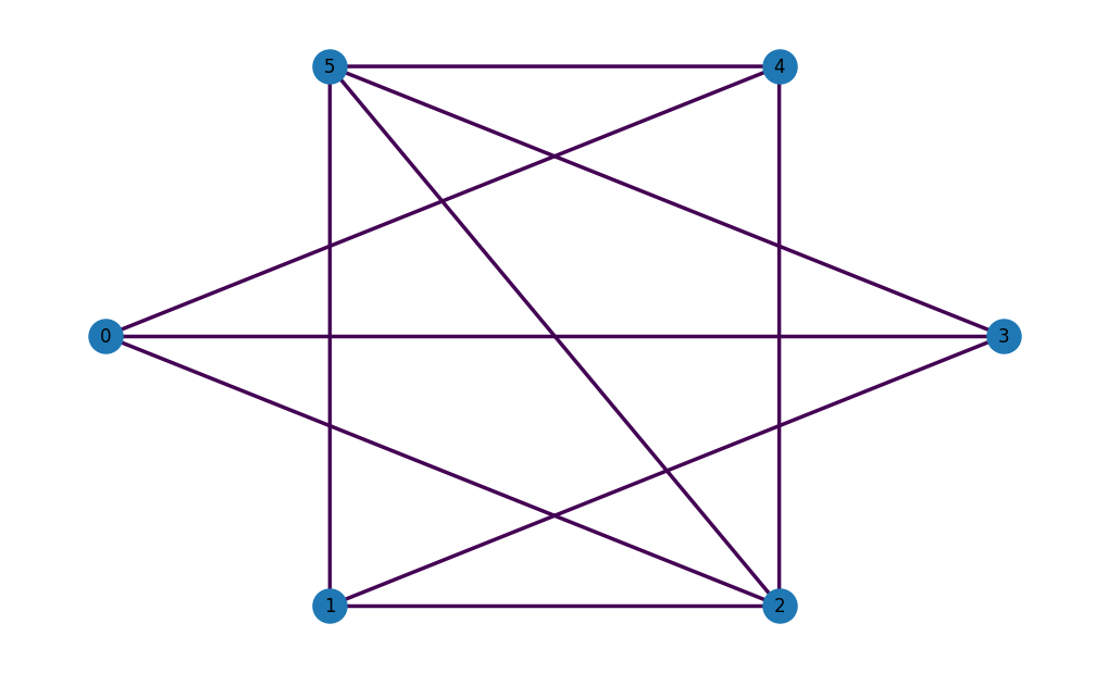
The Shortest Path problem being a graph problem, you can leverage the popular networkx to easily create a variety of graphs. For example, an Erdös-Rényi graph can be instantiated with

import networkx as nx

G = nx.generators.fast_gnp_random_graph(n=4, p=0.6, seed=42)
nx.set_edge_attributes(G, values = 1, name = 'weight')

Note

The Traveling Sales Person problem requires the graph edges to have associated weights.

OpenQAOA has a nice wrapper to plot networkx graphs

from openqaoa.utilities import plot_graph
plot_graph(G)

Once the graph is defined, creating a Traveling Salesman problem class requires only a few lines of code, specifying the constants values:

from openqaoa.problems import TSP

tsp_prob = TSP(G=G, A=10, B=1)
tsp_qubo = tsp_prob.qubo

We can then access the underlying cost hamiltonian

tsp_qubo.hamiltonian.expression

\[ -11.0Z_{3} - 13.25Z_{1} - 13.25Z_{2} - 13.25Z_{7} - 13.25Z_{8} - 15.5Z_{0} - 15.5Z_{4} - 15.5Z_{5} - 15.5Z_{6} + 0.25Z_{0}Z_{4} + 0.25Z_{0}Z_{5} + 0.25Z_{1}Z_{3} + 0.25Z_{2}Z_{3} + 0.25Z_{3}Z_{7} + 0.25Z_{3}Z_{8} + 0.25Z_{4}Z_{6} + 0.25Z_{5}Z_{6} + 2.5Z_{1}Z_{5} + 2.5Z_{2}Z_{4} + 2.5Z_{4}Z_{8} + 2.5Z_{5}Z_{7} + 5.0Z_{0}Z_{1} + 5.0Z_{0}Z_{2} + 5.0Z_{0}Z_{3} + 5.0Z_{0}Z_{6} + 5.0Z_{1}Z_{2} + 5.0Z_{1}Z_{4} + 5.0Z_{1}Z_{7} + 5.0Z_{2}Z_{5} + 5.0Z_{2}Z_{8} + 5.0Z_{3}Z_{4} + 5.0Z_{3}Z_{5} + 5.0Z_{3}Z_{6} + 5.0Z_{4}Z_{5} + 5.0Z_{4}Z_{7} + 5.0Z_{5}Z_{8} + 5.0Z_{6}Z_{7} + 5.0Z_{6}Z_{8} + 5.0Z_{7}Z_{8} + 84.0 \]

Note

The number of variables scales as \(\mathcal{O}(N^2)\)

You may also check all details of the problem instance in the form of a dictionary:

> tsp_qubo.asdict()

{'constant': 84.0,
 'metadata': {},
 'n': 9,
 'problem_instance': {'A': 10,
                      'B': 1,
                      'G': {'directed': True,
                            'graph': {},
                            'links': [{'source': 0, 'target': 2, 'weight': 1},
                                      {'source': 0, 'target': 3, 'weight': 1},
                                      {'source': 1, 'target': 2, 'weight': 1},
                                      {'source': 1, 'target': 3, 'weight': 1},
                                      {'source': 2, 'target': 0, 'weight': 1},
                                      {'source': 2, 'target': 1, 'weight': 1},
                                      {'source': 3, 'target': 0, 'weight': 1},
                                      {'source': 3, 'target': 1, 'weight': 1}],
                            'multigraph': False,
                            'nodes': [{'id': 0},
                                      {'id': 1},
                                      {'id': 2},
                                      {'id': 3}]},
                      'n_cities': 4,
                      'problem_type': 'tsp'},
 'terms': [[0, 3],
           [1, 4],
           [2, 5],
           [0, 6],
           [1, 7],
           [8, 2],
           [3, 6],
           [4, 7],
           [8, 5],
           [0, 1],
           [0, 2],
           [1, 2],
           [3, 4],
           [3, 5],
           [4, 5],
           [6, 7],
           [8, 6],
           [8, 7],
           [1, 5],
           [8, 4],
           [2, 4],
           [5, 7],
           [0, 4],
           [3, 7],
           [0, 5],
           [8, 3],
           [1, 3],
           [4, 6],
           [2, 3],
           [5, 6],
           [0],
           [1],
           [2],
           [3],
           [4],
           [5],
           [6],
           [7],
           [8]],
 'weights': [5.0, 5.0, 5.0, 5.0, 5.0, 5.0, 5.0, 5.0, 5.0, 5.0, 5.0, 5.0, 5.0, 5.0, 
             5.0, 5.0, 5.0, 5.0, 2.5, 2.5, 2.5, 2.5, 0.25, 0.25, 0.25, 0.25, 0.25,
             0.25, 0.25, 0.25, -15.5, -13.25, -13.25, -11.0, -15.5, -15.5, -15.5, 
             -13.25, -13.25]}