Shortest Path Problem
Given an undirected graph \(G(V,E)\), the shortest path problem for a given source \(s \in V\) and destination node \(d \in V\) seeks a path between them that has minimal distance. We consider the weighted variant of the problem, where nodes and edges of \(G\) are assigned node and edge weights. The distance of a path is then equal to the sum of node and edge weights along the path.
Mathematical Formulation
A QUBO encoding of the (weighted) shortest path problem can be constructed with \(|V| + |E| - 2\) binary variables. This is achieved by using linear terms to represent the node and edge weights, and quadratic penalty terms to penalize states that not valid paths, where a valid path is one that:
- starts from a specified source node \(s\),
- ends at a specified destination node \(d\), and
- has no broken links or branches along the path from \(s\) to \(d\).
In terms of binary variables \(\{0, 1\}\), the first \(|V|-2\) variables (denoted as \(x_i\), where \(i \in V\) corresponds to a node) correspond to nodes in the graph excluding the source and destination nodes, while the remaining \(|E|\) variables (denoted as \(x_{ij}\), where \((i,j) \in E\) represents an edge that is present in \(G\) between nodes \(i\) and \(j\)) represent the edges \(E\). A state \(\textbf{x}\) is then denoted as \(\textbf{x} = (x_1,..., x_{|V|-2},...,x_{ij},...)\). Note that this encoding implicitly specifies the starting and ending nodes, since they are always in the path.
Binary encoding
In this case it is much easier to write the cost function in terms onf \(\{0,1\}\) binary variables, and convert them to OpenQAOA ising encoding only at the end!
With this encoding, the QUBO cost function \(C(\textbf{x})\) can be written in the form:
\(C_w(\textbf{x})\) contains linear terms that encode the node and edge weights \(w_i\) and \(w_{ij}\) respectively:
while
contains linear and quadratic terms that enforce the conditions (1), (2), and (3) above. Explicitly, they are:
- 1 : Source constraint: Penalises paths that do not have exactly one edge connected to the source node with
where \(x_s = 1\), and the sum is over all edges that are connected to node \(s\). This term has a minimum value of \(-1\), which occurs for states where there is only one edge connected to the source node.
- 2 : Destination constraint: Penalises paths that do not have exactly one edge connected to the destination node with
where \(x_d = 1\), and the sum is over all edges that are connected to node \(d\). This term has a minimum value of \(-1\), which occurs for states where there is only one edge connected to the destination node.
- 3 : Path constraint: Penalises paths that do not have exactly 2 edges connected to intermediate nodes with
such that for every node \(i \in V\):
where the sum is over all edges that are connected to node \(i\). This has a minimum value of 0, which occurs for states where all nodes selected have exactly 2 edges connected to it.
States that minimize \(C_P(\textbf{x})\) then constitute valid paths that start at \(s\) and end at \(d\).
Note
In OpenQAOA, where we work with Ising variables \(\sigma_i\in\{-1,1\}\), a transformation of variables \(x_i \rightarrow (1-\sigma_i)/2\) transforms the cost function \(C(\textbf{x})\) to the QAOA cost Hamiltonian \(H\).
The Shortest Path Problem in OpenQAOA
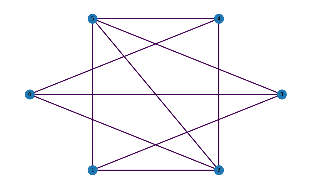
The Shortest Path problem being a graph problem, you can leverage the popular networkx to easily create a variety of graphs. For example, an Erdös-Rényi graph can be instantiated with
import networkx as nx

G = nx.generators.fast_gnp_random_graph(n=6, p=0.6, seed=42)
nx.set_edge_attributes(G, values = 1, name = 'weight')
nx.set_node_attributes(G, values = 1, name = 'weight')
Note
The Shortest Path problem requires the edges and nodes of the graph to have associated weights.
OpenQAOA has a nice wrapper to plot networkx graphs
Once the graph is defined, creating a Shortest Path problem class requires only a few lines of code, specifying which nodes are associated with the source and destination:
from openqaoa.problems import ShortestPath

sp_prob = ShortestPath(G, source=0, dest=5)
sp_qubo = sp_prob.qubo
We can then access the underlying cost hamiltonian
You may also check all details of the problem instance in the form of a dictionary:
> sp_qubo.asdict()

{'constant': 17.0,
 'metadata': {},
 'n': 14,
 'problem_instance': {'G': {'directed': False,
                            'graph': {},
                            'links': [{'source': 0, 'target': 2, 'weight': 1},
                                      {'source': 0, 'target': 3, 'weight': 1},
                                      {'source': 0, 'target': 4, 'weight': 1},
                                      {'source': 1, 'target': 2, 'weight': 1},
                                      {'source': 1, 'target': 3, 'weight': 1},
                                      {'source': 1, 'target': 5, 'weight': 1},
                                      {'source': 2, 'target': 4, 'weight': 1},
                                      {'source': 2, 'target': 5, 'weight': 1},
                                      {'source': 3, 'target': 5, 'weight': 1},
                                      {'source': 4, 'target': 5, 'weight': 1}],
                            'multigraph': False,
                            'nodes': [{'id': 0, 'weight': 1},
                                      {'id': 1, 'weight': 1},
                                      {'id': 2, 'weight': 1},
                                      {'id': 3, 'weight': 1},
                                      {'id': 4, 'weight': 1},
                                      {'id': 5, 'weight': 1}]},
                      'dest': 5,
                      'problem_type': 'shortest_path',
                      'source': 0},
 'terms': [[4, 5],
           [4, 6],
           [5, 6],
           [9, 11],
           [9, 12],
           [9, 13],
           [11, 12],
           [11, 13],
           [12, 13],
           [0, 7],
           [8, 7],
           [9, 7],
           [0, 8],
           [8, 9],
           [0, 9],
           [1, 4],
           [4, 7],
           [10, 4],
           [11, 4],
           [1, 7],
           [10, 7],
           [11, 7],
           [1, 10],
           [10, 11],
           [1, 11],
           [2, 5],
           [8, 5],
           [12, 5],
           [8, 2],
           [8, 12],
           [2, 12],
           [3, 6],
           [10, 6],
           [13, 6],
           [10, 3],
           [10, 13],
           [3, 13],
           [0],
           [1],
           [2],
           [3],
           [4],
           [5],
           [6],
           [7],
           [8],
           [9],
           [10],
           [11],
           [12],
           [13]],
 'weights': [0.5,
             0.5,
             0.5,
             0.5,
             0.5,
             0.5,
             0.5,
             0.5,
             0.5,
             -1.0,
             0.5,
             0.5,
             -1.0,
             0.5,
             -1.0,
             -1.0,
             0.5,
             0.5,
             0.5,
             -1.0,
             0.5,
             0.5,
             -1.0,
             0.5,
             -1.0,
             -1.0,
             0.5,
             0.5,
             -1.0,
             0.5,
             -1.0,
             -1.0,
             0.5,
             0.5,
             -1.0,
             0.5,
             -1.0,
             0.5,
             1.5,
             0.5,
             0.5,
             -2.0,
             -1.5,
             -1.5,
             -2.0,
             -1.5,
             -2.0,
             -2.0,
             -2.5,
             -2.0,
             -2.0]}