Annealing Parametrization

The QAOAVariationalAnnealingParams class implements a discretised form of quantum annealing.

In quantum annealing, we start in the ground state of a mixer Hamiltonian, \(H_M\), and gradually evolve to the ground state of a cost Hamiltonian, \(H_C\), according to some annealing schedule function \(s(t)\), where \(t\) denotes time. If it were possible to perform the transformation infinitesimally slowly, we would be guaranteed to arrive at the exact ground state of the cost Hamiltonian. In practice, the transformation is performed over some finite time, and we hope to prepare the ground state of \(H_C\) with some acceptably high probability.

At any time \(t\) during the procedure, the instantaneous Hamiltonian is given by

\[H(t) = \left(1 - s(t)\right)H_M + s(t)H_C\]

where \(s(0) = 0\), and \(s(t = T) = 1\), and \(T\) is the total annealing time.

Main difference

Unlike the other parametrizations for QAOA, in the annealing one the coefficients of the two Hamiltonians are necessarily related to one another: the mixer is applied with a weight \((1 - s(t))\), and the cost Hamiltonian with weight \(s(t)\).

The prepared quantum state is given by:

\[U = \mathcal{T}\left(\Pi_{j=1}^p \exp\left[-i(1-s(t_j)) H_M \Delta t\right]\exp\left[-i s(t_j) H_C \Delta t\right]\right),\]

where the object \(\mathcal{T}\) tells us to correctly order the terms, increasing from \(j=1\) to \(j=p\) from right to left in the product.

For the curious

It is common to view the QAOA as a form of discretised annealing, where the procedure is performed in a fixed number of steps, \(p\). However, the coefficients of the mixer and cost Hamiltonians need not be related in the simple way that they are in a conventional annealing schedule.

Let us now go through a simple example using the same cost Hamiltonian as in the other sections, namely

\[ H_C = 2.5 (Z_0Z_1 + Z_1Z_2 + Z_0Z_2) + 3.5 (Z_0 + Z_1 + Z_2). \]

We can use the annealing parametrization with ramp initialization by using

q = QAOA()

q.set_circuit_properties(p=2, 
                         param_type='annealing', 
                         init_type='ramp')

The schedule, \(s(t)\), when using ramp is an array of equally spaced numbers from \(0.5\) to \(1-0.5\) divided by the number of layers, p. For example, for the code excerpt from above, the schedule is \([0.25, 0.75]\). The total annealing time is a multiple of p, i.e. \(T = \Delta t * p\).

Unless specified explicitly, \(\Delta t = 0.7\)

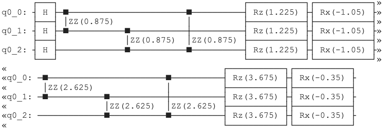
The parameters of the circuit are then \(\gamma_i = s(t_i) * \Delta t\) and \(\beta_i = (1 - s(t_i)) * \Delta t\). Multiplying by the weights and biases of the hamiltonian where relevant, we end up with the following circuit:

Supported initializations

Only ramp and rand initializations are supported in this class. Note that custom will result in an error.