Recursive QAOA¶

In this notebook, we provide a short introduction to recursive QAOA, and demonstrate how this technique is implemented in the OpenQAOA workflows, by solving the Sherrington-Kirkpatrick Hamiltonian with \(\pm1\) weights.

A brief introduction to RQAOA¶

Recursive QAOA (RQAOA) is an iterative variant of QAOA, first introduced by Bravyi et. al in [1] and further explored in [2,3].

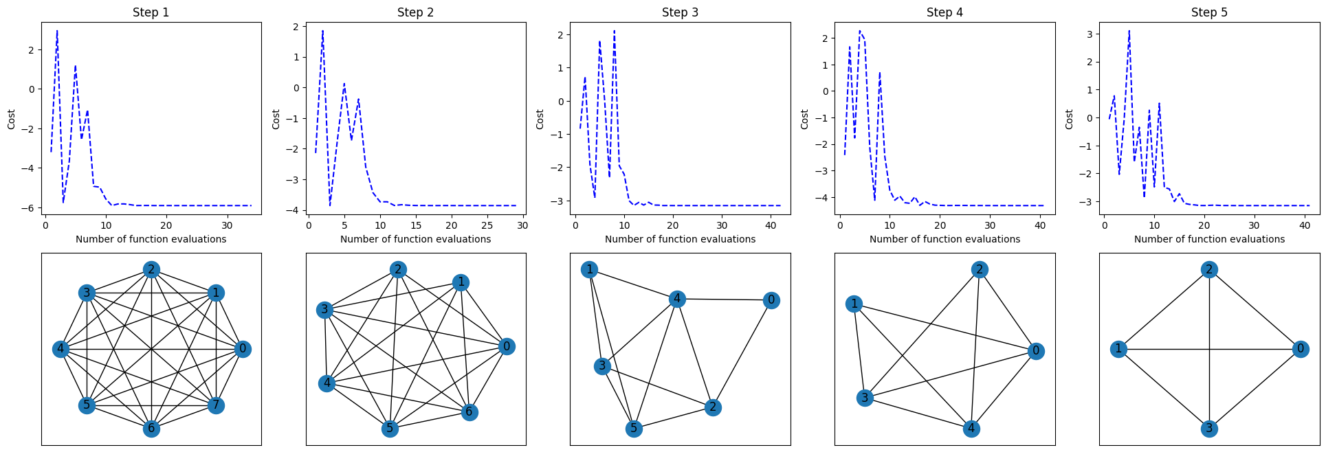
This technique consists in recursively reducing the size of the problem by running QAOA. At each step, the QAOA output distribution is used to compute the expectation values

\[ \mathcal{M}_{i} = \langle Z_{i} \rangle \qquad \qquad \qquad \qquad \qquad \mathcal{M}_{ij} = \langle Z_{i}Z_{j} \rangle, \]

associated with the terms present in the Hamiltonian. Note that, by definition, these quantities are bounded between -1 and 1. The expectation values are then ranked according to their magnitude \(|\mathcal{M}_{(i,ij)}|\). In its original formulation, the highest ranked value is selected. This value is then utilized to eliminate a qubit from the Hamiltonian. This is done by first, performing integer rounding of the expectation value, i.e. \(\mathcal{M}_{(i,ij)} \rightarrow \textrm{sign}(\mathcal{M}_{(i,ij)})\), then transforming the rounded value into a constraint on the respective\ qubits

\[ Z_{i} \rightarrow \textrm{sign}(\mathcal{M}_{(i)}) \qquad \qquad \qquad \qquad \qquad \langle Z_{i} Z_{j} \rangle \rightarrow \textrm{sign}(\mathcal{M}_{(ij)}), \]

and last, inserting the constraint into the Hamiltonian, effectively reducing the size of the problem by one qubit. Using the reduced Hamiltonian, QAOA is run again and the same procedure is followed. Once the reduced problem reaches a predefined cutoff size, it is solved exactly via classical methods. The final answer is then reconstructed by re-inserting the eliminated qubits into the classical solution following the appropriate order.

This version of RQAOA is included in OpenQAOA. Additionally, OpenQAOA incorporates RQAOA from two different generalized version of these procedure, which enable multiple qubit eliminations during the recursive process. These strategies are denoted as custom and adaptive [4], in accordance with the precise concept under which the elimination method takes place. In a nutshell, they are described as follows:

The custom strategy allows the user to define the number of eliminations to be performed at each step. This defined by the parameter steps. If the parameter is set as an integer, the algorithm will use this value as the number of qubits to be eliminated at each step. Alternatively, it is possible to pass a list, which specifies the number of qubits to be eliminated at each step. For steps=1, the algorithm reduces to the original form of RQAOA presented in [1].
The adaptive strategy selects how many qubits to eliminate at each step adaptively. The maximum number of allowed eliminations is given by the parameter n_max. At each step, the algorithm selects the top n_max+1 expectation values (ranked in magnitude), computes the mean among them, and uses the ones lying above it for qubit elimination. This corresponds to a maximum of n_max possible elimination per step. For n_max=1, the algorithm reduces to the original form of RQAOA presented in [1].

Active Research

The specific performance of these generalizations is currently under investigation. In particular, the development of Adaptive RQAOA is associated with an internal research project at Entropica Labs to be released publicly in the near future [4]. We make these strategies already available to the community in order to strengthen the exploration of more complex elimination schemes for RQAOA, beyond its original formulation [1].

The full RQAOA workflow.¶

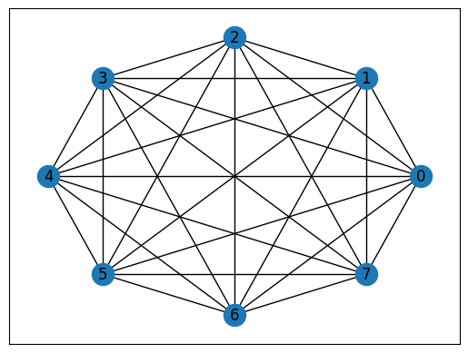
Let us now do a walk through the whole process using the Sherrington-Kirkpatrick model as an example. This model corresponds to a fully-connected system, where we choose the couplings \(J_{ij}\) to be of magnitude 1, but with randomly assigned signs. Then we have to translate the problem to a Quadratic Unconstrained Binary Optimization problem. This can be done in a single line by creating an object of the class QUBO which takes the number of qubits, connectivity of the problem (terms) and the couplings (weights).

import networkx as nx
from openqaoa import QUBO

# Number of qubits
n_qubits = 8

# Define fully-connected terms
terms = [(i,j) for j in range(n_qubits) for i in range(j)]

# Assign coupling signs at random
rng = np.random.default_rng(42)
weights = [(-1)**np.round(rng.random()) for _ in range(len(terms))]

# Define QUBO problem
sk = QUBO(n_qubits,terms,weights)

# Plot geometry
sk_graph = nx.Graph()
sk_graph.add_edges_from(terms)
nx.draw_networkx(sk_graph, pos = nx.kamada_kawai_layout(sk_graph))

The underlying graph for this problem

kamada_kawai_layout

We now demonstrate the full RQAOA workflow.

from openqaoa import RQAOA, create_device

r =  RQAOA()

# Set up RQAOA properties
n_cutoff = 3 # Cutoff size at which to solve things classically
n_steps = 1 # Number of eliminations per step

# Set instance parameters
r.set_rqaoa_parameters(n_cutoff=n_cutoff, steps=n_steps, rqaoa_type='custom')

# Set the properties you want - These values are actually the default ones!
r.set_circuit_properties(p=1, param_type='standard', init_type='ramp', mixer_hamiltonian='x')
r.set_classical_optimizer(method='cobyla', maxiter=200, tol=0.001)

device = create_device(location='local', name='vectorized')
r.set_device(device)

r.compile(sk)
r.optimize()

The RQAOA result object¶

The results show the final solution of the problem, the output from the classical solution on the reduced problem, the set of eliminations performed (on which pair and which correlation), the schedule followed (the number of eliminations at each step), the total number of recursive steps it took to reach the cutoff size and the all the information regarding the problem and QAOA run in the intermediate steps.

{'solution': {'10001000': -12.0, '01110111': -12.0},
 'classical_output': {'minimum_energy': -3.0,
  'optimal_states': ['100', '011']},
 'elimination_rules': [[{'pair': (2, 4), 'correlation': -1.0}],
  [{'pair': (0, 4), 'correlation': -1.0}],
  [{'pair': (0, 4), 'correlation': -1.0}],
  [{'pair': (2, 3), 'correlation': 1.0}],
  [{'pair': (2, 3), 'correlation': 1.0}]],
 'schedule': [1, 1, 1, 1, 1],
 'number_steps': 5,
 'intermediate_steps': [{'counter': 0,
   'problem': <openqaoa.problems.qubo.QUBO at 0x7f39b341f460>,
   'qaoa_results': <openqaoa.optimizers.result.Result at 0x7f3a13dfb7f0>,
   'exp_vals_z': array([0., 0., 0., 0., 0., 0., 0., 0.]),
   'corr_matrix': array([[ 0.        ,  0.12081413, -0.2361811 ,  0.04850827,  0.29105518,
           -0.2361811 , -0.12081413, -0.18130702],
          [ 0.        ,  0.        ,  0.18130702, -0.12081413,  0.2361811 ,
            0.18130702,  0.18130702,  0.12081413],
          [ 0.        ,  0.        ,  0.        ,  0.2361811 , -0.35154807,
            0.29105518, -0.18130702,  0.35154807],
          [ 0.        ,  0.        ,  0.        ,  0.        , -0.29105518,
            0.2361811 ,  0.12081413,  0.18130702],
          [ 0.        ,  0.        ,  0.        ,  0.        ,  0.        ,
           -0.2361811 ,  0.2361811 , -0.29105518],
          [ 0.        ,  0.        ,  0.        ,  0.        ,  0.        ,
            0.        ,  0.29105518, -0.12081413],
          [ 0.        ,  0.        ,  0.        ,  0.        ,  0.        ,
            0.        ,  0.        , -0.2361811 ],
          [ 0.        ,  0.        ,  0.        ,  0.        ,  0.        ,
            0.        ,  0.        ,  0.        ]])},
  {'counter': 1,
   'problem': <openqaoa.problems.qubo.QUBO at 0x7f3a4bbf0b20>,
   'qaoa_results': <openqaoa.optimizers.result.Result at 0x7f3a4bbf04f0>,
   'exp_vals_z': array([0., 0., 0., 0., 0., 0., 0.]),
   'corr_matrix': array([[ 0.        ,  0.12149926, -0.16779332, -0.03100176, -0.25414406,
           -0.03937175, -0.24998213],
          [ 0.        ,  0.        ,  0.        , -0.12149926,  0.18034528,
            0.18034528,  0.12149926],
          [ 0.        ,  0.        ,  0.        ,  0.16779332,  0.16779332,
           -0.19795548,  0.13763115],
          [ 0.        ,  0.        ,  0.        ,  0.        ,  0.25414406,
            0.03937175,  0.24998213],
          [ 0.        ,  0.        ,  0.        ,  0.        ,  0.        ,
            0.1050155 , -0.03937175],
          [ 0.        ,  0.        ,  0.        ,  0.        ,  0.        ,
            0.        , -0.25414406],
          [ 0.        ,  0.        ,  0.        ,  0.        ,  0.        ,
            0.        ,  0.        ]])},
  {'counter': 2,
   'problem': <openqaoa.problems.qubo.QUBO at 0x7f39b333d1b0>,
   'qaoa_results': <openqaoa.optimizers.result.Result at 0x7f39b333da50>,
   'exp_vals_z': array([0., 0., 0., 0., 0., 0.]),
   'corr_matrix': array([[ 0.        ,  0.        ,  0.16085035,  0.        , -0.62390462,
            0.        ],
          [ 0.        ,  0.        ,  0.        , -0.17543822,  0.18647518,
            0.17543822],
          [ 0.        ,  0.        ,  0.        ,  0.29324292, -0.06223818,
            0.39421389],
          [ 0.        ,  0.        ,  0.        ,  0.        , -0.01269842,
            0.36664087],
          [ 0.        ,  0.        ,  0.        ,  0.        ,  0.        ,
           -0.16107545],
          [ 0.        ,  0.        ,  0.        ,  0.        ,  0.        ,
            0.        ]])},
  {'counter': 3,
   'problem': <openqaoa.problems.qubo.QUBO at 0x7f39b32f3190>,
   'qaoa_results': <openqaoa.optimizers.result.Result at 0x7f39b32f3b20>,
   'exp_vals_z': array([0., 0., 0., 0., 0.]),
   'corr_matrix': array([[ 0.        , -0.18916614, -0.45557513, -0.35756255, -0.02233763],
          [ 0.        ,  0.        ,  0.        , -0.18916614,  0.18916614],
          [ 0.        ,  0.        ,  0.        ,  0.6210754 ,  0.45557513],
          [ 0.        ,  0.        ,  0.        ,  0.        ,  0.35756255],
          [ 0.        ,  0.        ,  0.        ,  0.        ,  0.        ]])},
  {'counter': 4,
   'problem': <openqaoa.problems.qubo.QUBO at 0x7f39b32f2260>,
   'qaoa_results': <openqaoa.optimizers.result.Result at 0x7f39b32f2c80>,
   'exp_vals_z': array([0., 0., 0., 0.]),
   'corr_matrix': array([[ 0.        , -0.12297744, -0.47157466, -0.01462733],
          [ 0.        ,  0.        , -0.08821626,  0.12297744],
          [ 0.        ,  0.        ,  0.        ,  0.47157466],
          [ 0.        ,  0.        ,  0.        ,  0.        ]])}],
 'atomic_uuids': {0: 'e62903c6-0c2c-4637-b352-3fd473fc674a',
  1: '9fbc9ad5-d218-4d5a-9a04-ca6fd46877c5',
  2: '6b110d3d-56cf-4fa4-aa2d-6b0d73771fe4',
  3: '75e5d135-c1ea-4964-8c90-df84727e0bc6',
  4: '479c9f4a-db8c-412e-89ed-b42725876f56'}}

From the intermediate steps, we can extract useful properties such as the cost optimization, the shape of the system, or the correlation matrix at that step. The r.result object has some methods that help to get the intermediate steps: .get_qaoa_results(step), .get_problem(step), plot_corr_matrix(step), among my others (see documentation [ADD LINK]).

kamada_kawai_layout

References¶

S. Bravyi, A. Kliesch, R. Koenig, and E. Tang, Physical Review Letters 125, 260505 (2020)
S. Bravyi, A. Kliesch, R. Koenig, and E. Tang, (2020), 10.22331/q-2022-03-30-678
D. J. Egger, J. Marecek, and S. Woerner, Quantum 5, 479 (2021)
E. I. Rodríguez Chiacchio, V. Sharma, E. Munro (Work in progress)