What is a QUBO?
QAOA can solve binary optimization problems known as QUBOs. QUBO stands for Quadratic unconstrained binary optimization, and a QUBO problem represent, loosely speaking, a binary problem with at most quadratic terms. In general any optimization problem can be cast as a binary problem, but not all of them will be quadratic in the resulting binary variables. For a very nice paper showcasing the QUBO formulation of most common optimization problems, please check out Andrew Lucas's paper Ising formulations of many NP problems
Binary optimization
Binary optimization is a type of combinatorial optimization problem in which the variables are limited to two values. For example, a variable \(x\) can be either 0 or 1. A binary optimization problem then reflect the effort of minimizing a cost function \(C(\textbf{x})\) of \(n\) variables, where \(\textbf{x} =(x_1, \dots, x_n)^\top\) is a vector collecting all variables.
In its most general form, a binary optimization problem can be written as
{0,1} or {-1,+1}
In OpenQAOA we always use the \(\{-1, +1\}\) encoding (also known as the Ising encoding).
How to write a QUBO
For our needs, we will be limiting ourself to Quadratic Unconstrained Binary Optimization (QUBO) problems. These problems are binary optimization problems which features at most most polynomial of order 2.
The most general formulation of a QUBO is then
where \(x_i \in\{0, 1\}\) are the binary variables and \(Q_{ij}\) represents the quadratic coefficients. We note that the cost function can in principle also include a constant term, but this will not change which configuration minimizes \(C(\cdot)\).
In the context of QAOA, we will be interested in the equivalent formulation known as Ising model, where the cost function is
where \(\sigma_i \in\{-1, 1\}\) are Ising variables and \(h_i\) and \(J_{ij}\) represent the coefficients for the linear and quadratic coefficients.
From QUBO to Ising Model and Back
One can easily convert a QUBO problem to an equivalent Ising formulation by subtituting each \(x_i\) with \(\frac{1+\sigma_i}{2}\). Similarly, one can convert an Ising problem to an equivalent QUBO formulation by subtituting each \(\sigma_i\) with \(2x_i-1\).
The following equation shows an example of a QUBO problem involving three variables
as you can see, we only have linear and quadratic terms in \(x\).
From QUBOs to QAOA
As explained in the what-is-the-qaoa page, QUBOs are used in QAOA to build the Cost Hamiltonian. There are two important points worth mentioning explicitly:
- The QUBO can be represented by a weighted graph \(G(V,E)\) defined by \(V\) vertexes and \(E\) edges, where the linear part of the QUBO represent the weight of the vertexes and the quadratic is the weight associated to the edges,
- The QAOA cost function should be defined as an Ising model, that is, variables should take values in \(\{ -1, 1\}\). This means that if one has a QUBO formulation which assumes variables to be in \(\{0,1\}\), a conversion must take place to retrieve the equivalent problem but with variables in \(\{-1, 1\}\).
QUBOs in OpenQAOA
A QUBO in OpenQAOA is simply described by two lists, and a number for the constant constant term. Using the example above with
the corresponding initialization in OpenQAOA looks like
terms = [[0], [1], [0,1], [1,2], [0,2]]
weights = [3, 2, 6, 4, 5]
qubo = QUBO(n=3, terms=terms, weights=weights)
Python index
Remember that in python indexes start at zero!
Creating the OpenQAOA QUBO is simple
if we then check the dictionary representation of our qubo we get
{'terms': [[0], [1], [0, 1], [1, 2], [0, 2]],
 'weights': [3.0, 2.0, 6.0, 4.0, 5.0],
 'constant': 0,
 'n': 3,
 'problem_instance': {'problem_type': 'generic_qubo'},
 'metadata': {}}
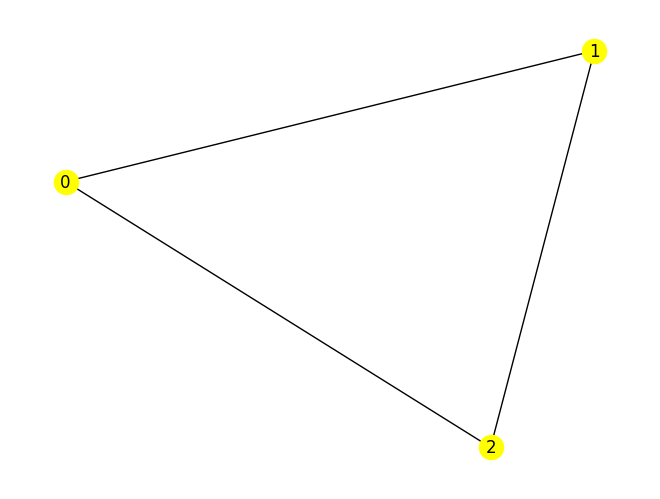
QUBOs can also be nicely represented as weighted graphs: the terms contains the list of vertices (the linear terms) and the edges (the quadratic terms), and the weight represent the weight of each vertex or edge.
To retrieve such a graph within OpenQAOA, simply type
import networkx as nx

networkx_graph = utilities.graph_from_hamiltonian(qubo.hamiltonian)
nx.draw(networkx_graph, with_labels=True, node_color='yellow')
We also obtain the underlying cost hamiltonian by executing